Inference with xgboost
Source:vignettes/articles/Inference-with-xgboost.Rmd
Inference-with-xgboost.RmdThis article contains a workflow in R to analyze a data set using xgboost to get insights that can help a consultant make important business decisions.
knitr::opts_chunk$set(warning = FALSE, message = FALSE)
library(pacman)
library(tidyverse); library(EIX); library(validata); p_load(TidyConsultant)
set.seed(1)
Inspect data set
We will use the HR_data from the EIX package. Let’s inspect the variables using the validata package.
HR_data
#>        satisfaction_level last_evaluation number_project average_montly_hours
#>                     <num>           <num>          <int>                <int>
#>     1:               0.38            0.53              2                  157
#>     2:               0.80            0.86              5                  262
#>     3:               0.11            0.88              7                  272
#>     4:               0.72            0.87              5                  223
#>     5:               0.37            0.52              2                  159
#>    ---
#> 14995:               0.40            0.57              2                  151
#> 14996:               0.37            0.48              2                  160
#> 14997:               0.37            0.53              2                  143
#> 14998:               0.11            0.96              6                  280
#> 14999:               0.37            0.52              2                  158
#>        time_spend_company Work_accident  left promotion_last_5years   sales
#>                     <int>         <int> <int>                 <int>  <fctr>
#>     1:                  3             0     1                     0   sales
#>     2:                  6             0     1                     0   sales
#>     3:                  4             0     1                     0   sales
#>     4:                  5             0     1                     0   sales
#>     5:                  3             0     1                     0   sales
#>    ---
#> 14995:                  3             0     1                     0 support
#> 14996:                  3             0     1                     0 support
#> 14997:                  3             0     1                     0 support
#> 14998:                  4             0     1                     0 support
#> 14999:                  3             0     1                     0 support
#>        salary
#>        <fctr>
#>     1:    low
#>     2: medium
#>     3: medium
#>     4:    low
#>     5:    low
#>    ---
#> 14995:    low
#> 14996:    low
#> 14997:    low
#> 14998:    low
#> 14999:    low
HR_data %>%
  diagnose_category(max_distinct = 100)
#> # A tibble: 13 × 4
#>    column level           n  ratio
#>    <chr>  <fct>       <int>  <dbl>
#>  1 sales  sales        4140 0.276
#>  2 sales  technical    2720 0.181
#>  3 sales  support      2229 0.149
#>  4 sales  IT           1227 0.0818
#>  5 sales  product_mng   902 0.0601
#>  6 sales  marketing     858 0.0572
#>  7 sales  RandD         787 0.0525
#>  8 sales  accounting    767 0.0511
#>  9 sales  hr            739 0.0493
#> 10 sales  management    630 0.0420
#> 11 salary low          7316 0.488
#> 12 salary medium       6446 0.430
#> 13 salary high         1237 0.0825
HR_data %>%
  diagnose_numeric()
#> # A tibble: 8 × 10
#>   variables   zeros minus infs    min  mean   max `|x|<=1 (ratio)` integer_ratio
#>   <chr>       <chr> <chr> <chr> <int> <int> <int> <chr>            <chr>
#> 1 satisfacti… 0 (0… 0 (0… 0 (0…     0     0     1 14999 (100%)     111 (1%)
#> 2 last_evalu… 0 (0… 0 (0… 0 (0…     0     0     1 14999 (100%)     283 (2%)
#> 3 number_pro… 0 (0… 0 (0… 0 (0…     2     3     7 0 (0%)           14999 (100%)
#> 4 average_mo… 0 (0… 0 (0… 0 (0…    96   201   310 0 (0%)           14999 (100%)
#> 5 time_spend… 0 (0… 0 (0… 0 (0…     2     3    10 0 (0%)           14999 (100%)
#> 6 Work_accid… 1283… 0 (0… 0 (0…     0     0     1 14999 (100%)     14999 (100%)
#> 7 left        1142… 0 (0… 0 (0…     0     0     1 14999 (100%)     14999 (100%)
#> 8 promotion_… 1468… 0 (0… 0 (0…     0     0     1 14999 (100%)     14999 (100%)
#> # ℹ 1 more variable: mode <chr>
xgboost binary classification model
Create dummy variables out of the Sales and Salary column. We will
predict whether an employee left the company using xgboost. For this
reason, set left = 1 to the first level of the factor, so
it will be treated as the event class. A high predicted indicates a
label of the event class.
HR_data %>%
  framecleaner::create_dummies() %>%
  framecleaner::set_fct(left, first_level = "1") -> hr1
Create the model using xgboost. Since the goal of this model is to run inference using trees, we want to set tree_depth to 2 to make easily-interpretable trees.
When the model is run, feature importance on the full data is printed. Also the data is split into train and test, where the accuracy is calculated on a test set. Since this is a binary classification problem, a confusion matrix is output along with binary metrics.
hr1 %>%
  tidy_formula(left) -> hrf

hr1 %>%
  tidy_xgboost(hrf, tree_depth = 2L, trees = 100L, mtry = .75) -> xg1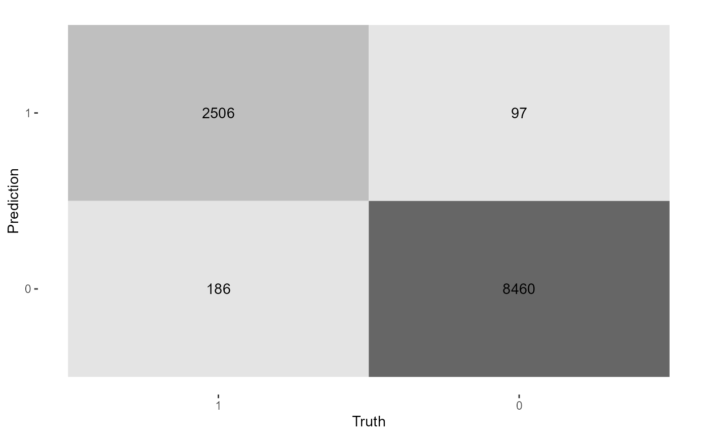
#> # A tibble: 15 × 3
#>    .metric              .estimate .formula
#>    <chr>                    <dbl> <chr>
#>  1 accuracy                 0.958 TP + TN / total
#>  2 kap                      0.883 NA
#>  3 sens                     0.871 TP / actually P
#>  4 spec                     0.986 TN / actually N
#>  5 ppv                      0.953 TP / predicted P
#>  6 npv                      0.960 TN / predicted N
#>  7 mcc                      0.884 NA
#>  8 j_index                  0.857 NA
#>  9 bal_accuracy             0.928 sens + spec / 2
#> 10 detection_prevalence     0.221 predicted P / total
#> 11 precision                0.953 PPV, 1-FDR
#> 12 recall                   0.871 sens, TPR
#> 13 f_meas                   0.910 HM(ppv, sens)
#> 14 baseline_accuracy        0.758 majority class / total
#> 15 roc_auc                  0.977 NA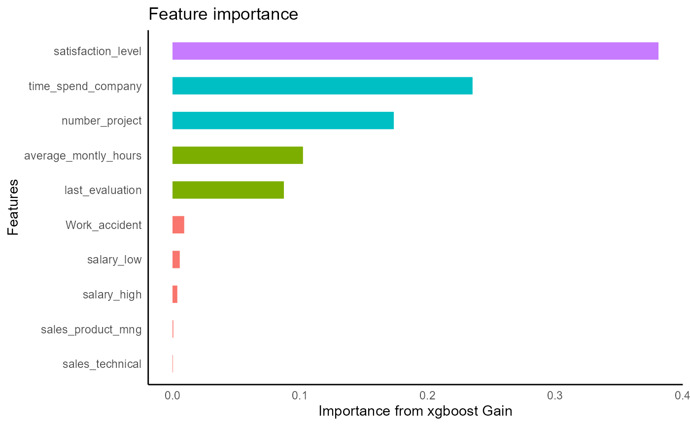
This line will save the tree structure of the model as a table.
xg1 %>%
xgboost::xgb.model.dt.tree(model = .)  -> xg_trees

xg_trees
#>       Tree  Node     ID              Feature  Split    Yes     No Missing
#>      <int> <int> <char>               <char>  <num> <char> <char>  <char>
#>   1:     0     0    0-0 average_montly_hours 288.00    0-1    0-2     0-2
#>   2:     0     1    0-1   satisfaction_level   0.47    0-3    0-4     0-4
#>   3:     0     2    0-2                 Leaf     NA   <NA>   <NA>    <NA>
#>   4:     0     3    0-3                 Leaf     NA   <NA>   <NA>    <NA>
#>   5:     0     4    0-4                 Leaf     NA   <NA>   <NA>    <NA>
#>  ---
#> 608:    99     2   99-2 average_montly_hours 162.00   99-5   99-6    99-6
#> 609:    99     3   99-3                 Leaf     NA   <NA>   <NA>    <NA>
#> 610:    99     4   99-4                 Leaf     NA   <NA>   <NA>    <NA>
#> 611:    99     5   99-5                 Leaf     NA   <NA>   <NA>    <NA>
#> 612:    99     6   99-6                 Leaf     NA   <NA>   <NA>    <NA>
#>               Gain      Cover
#>              <num>      <num>
#>   1:  8.012269e+02 2056.34204
#>   2:  2.794244e+03 2010.99219
#>   3:  2.076119e-01   45.34982
#>   4:  9.449380e-02  532.40680
#>   5: -3.902787e-02 1478.58533
#>  ---
#> 608:  6.358565e+01 1055.31921
#> 609: -8.300844e-02   14.49944
#> 610: -5.473283e-02   18.97126
#> 611:  2.040233e-02  342.93545
#> 612: -5.765188e-03  712.38373
Let’s plot the first tree and interpret the table output. For tree=0, the root feature (node=0) is satisfaction level, which is split at value .465. Is satisfaction_level < .465? If Yes, observations go left to node 1, if no, observations go right to node 2. Na values would go to node 1 if present. The quality of the split is represented by its Gain: 3123, the improvement in training loss.
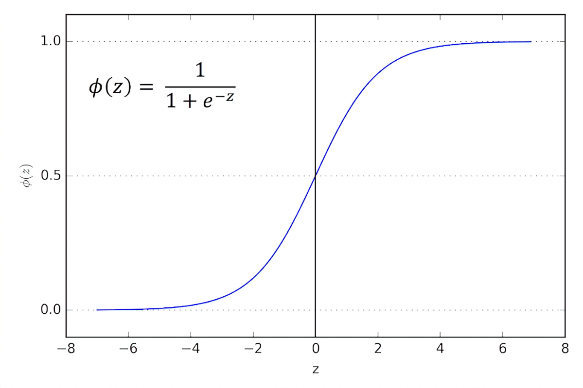
xgboost::xgb.plot.tree(model = xg1, trees = 0)The quality in the leaves is the prediction for observations in those leaves represented by log odds. To interpret them as probabilities, use the function below. Importantly, a log odds of 0 is a 0.5 probability.
Analyze interactions
In xgboost, an interaction occurs when the downstream split has a higher gain than the upstream split.
# write the function collapse_tree to convert the tree output to interactions that occur in the tree.

collapse_tree <- function(t1){

t1 %>% group_by(Tree) %>% slice(which(Node == 0)) %>% ungroup %>%
  select(Tree,  Root_Feature = Feature) %>%
  bind_cols(

    t1 %>% group_by(Tree) %>%  slice(which(Node == 1)) %>% ungroup %>%
      select(Child1 = Feature)
  ) %>%
  bind_cols(

    t1 %>% group_by(Tree) %>% slice(which(Node == 2)) %>% ungroup %>%
      select(Child2 = Feature)
  ) %>%
  unite(col = "interaction1", Root_Feature, Child1, sep = ":", remove = F) %>%
  select(-Child1) %>%
  unite(col = "interaction2", Root_Feature, Child2, sep = ":", remove = T) %>%
  pivot_longer(names_to = "names", cols = matches("interaction"), values_to = "interactions") %>%
    select(-names)
}

xg_trees %>%
  collapse_tree -> xg_trees_interactions
find the top interactions in the model. The interactions are rated with different importance metrics, ordered by sumGain.
imps <- EIX::importance(xg1, hr1, option = "interactions")
as_tibble(imps) %>%
  set_int(where(is.numeric))
#> # A tibble: 19 × 7
#>    Feature               sumGain sumCover meanGain meanCover frequency mean5Gain
#>    <chr>                   <int>    <int>    <int>     <int>     <int>     <int>
#>  1 satisfaction_level:n…    6818    24230      401      1425        17       691
#>  2 satisfaction_level:t…    5709     9017      713      1127         8       968
#>  3 average_montly_hours…    2794     2011     2794      2011         1      2794
#>  4 number_project:satis…    2688     3906      896      1302         3       896
#>  5 time_spend_company:s…    1991     2573      995      1286         2       995
#>  6 average_montly_hours…    1493     3264      298       652         5       298
#>  7 average_montly_hours…    1179     2483      392       827         3       392
#>  8 last_evaluation:time…    1171     2589      292       647         4       292
#>  9 last_evaluation:numb…    1003     3180      334      1060         3       334
#> 10 last_evaluation:sati…     904     6079      150      1013         6       163
#> 11 time_spend_company:l…     601      388      601       388         1       601
#> 12 last_evaluation:aver…     578      526      578       526         1       578
#> 13 number_project:last_…     431     1222      215       611         2       215
#> 14 satisfaction_level:a…     311     1772      155       885         2       155
#> 15 average_montly_hours…     290      606      290       606         1       290
#> 16 number_project:time_…     164      365      164       365         1       164
#> 17 Work_accident:time_s…     123     1144      123      1144         1       123
#> 18 satisfaction_level:l…      81     1115       81      1115         1        81
#> 19 time_spend_company:s…      75     1023       75      1023         1        75
We can extract all the trees that contain the specified interaction.
imps[1,1] %>% unlist -> top_interaction


xg_trees_interactions %>%
  filter(str_detect(interactions, top_interaction)) %>%
  distinct -> top_interaction_trees

top_interaction_trees
#> # A tibble: 23 × 2
#>     Tree interactions
#>    <int> <chr>
#>  1     2 satisfaction_level:number_project
#>  2     4 satisfaction_level:number_project
#>  3     7 satisfaction_level:number_project
#>  4    11 satisfaction_level:number_project
#>  5    12 satisfaction_level:number_project
#>  6    16 satisfaction_level:number_project
#>  7    17 satisfaction_level:number_project
#>  8    18 satisfaction_level:number_project
#>  9    19 satisfaction_level:number_project
#> 10    20 satisfaction_level:number_project
#> # ℹ 13 more rows
Then extract the first 3 (most important) trees and print them.
top_interaction_trees$Tree %>% unique %>% head(3) -> trees_index


xgboost::xgb.plot.tree(model = xg1, trees = trees_index)
We can confirm they are interactions because the child leaf in the interaction has higher split gain than the root leaf.
Analyze single features
# EIX package gives more detailed importances than the standard xgboost package
imps_single <- EIX::importance(xg1, hr1, option = "variables")

# choose the top feature
imps_single[1, 1] %>% unlist -> feature1

# get the top 3 rees of the most important feature. Less complicated than with interactions so
# no need to write a separate function like collapse tree
xg_trees %>%
  group_by(Tree) %>%
  slice(which(Node == 0)) %>%
  ungroup %>%
  filter(Feature %>% str_detect(feature1)) %>%
  distinct(Tree) %>%
  slice(1:3) %>%
  unlist -> top_trees

xgboost::xgb.plot.tree(model = xg1, trees = top_trees)
By looking at the 3 most important splits for satisfaction_level we can get a sense of how its splits affect the outcome.
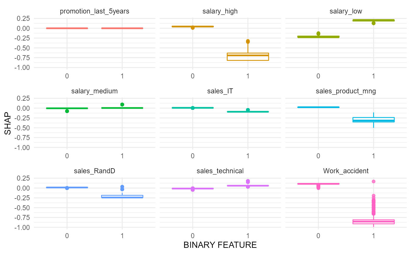
shapley values
xg1 %>%
  tidy_shap(hr1, form = hrf) -> hr_shaps

hr_shaps
#> $shap_tbl
#> # A tibble: 14,999 × 21
#>    satisfaction_level last_evaluation number_project average_montly_hours
#>                 <dbl>           <dbl>          <dbl>                <dbl>
#>  1              1.04           0.0302          1.30                0.0846
#>  2             -0.350          0.362          -0.294               0.213
#>  3              3.63           0.195          -0.264               0.142
#>  4             -0.380          0.364          -0.321               0.0841
#>  5              1.04           0.0302          1.30                0.0564
#>  6              1.04           0.0302          1.30                0.0846
#>  7              3.66          -0.147          -0.290               0.123
#>  8             -0.349          0.364          -0.294               0.213
#>  9             -0.326          0.797          -0.316               0.0841
#> 10              1.04           0.0302          1.30                0.0846
#> # ℹ 14,989 more rows
#> # ℹ 17 more variables: time_spend_company <dbl>, Work_accident <dbl>,
#> #   promotion_last_5years <dbl>, sales_accounting <dbl>, sales_hr <dbl>,
#> #   sales_it <dbl>, sales_management <dbl>, sales_marketing <dbl>,
#> #   sales_product_mng <dbl>, sales_rand_d <dbl>, sales_sales <dbl>,
#> #   sales_support <dbl>, sales_technical <dbl>, salary_high <dbl>,
#> #   salary_low <dbl>, salary_medium <dbl>, `(Intercept)` <dbl>
#>
#> $shaps_long
#> # A tibble: 314,979 × 3
#>    name         SHAP FEATURE
#>    <chr>       <dbl>   <dbl>
#>  1 (Intercept) -1.18      NA
#>  2 (Intercept) -1.18      NA
#>  3 (Intercept) -1.18      NA
#>  4 (Intercept) -1.18      NA
#>  5 (Intercept) -1.18      NA
#>  6 (Intercept) -1.18      NA
#>  7 (Intercept) -1.18      NA
#>  8 (Intercept) -1.18      NA
#>  9 (Intercept) -1.18      NA
#> 10 (Intercept) -1.18      NA
#> # ℹ 314,969 more rows
#>
#> $shap_summary
#> # A tibble: 21 × 5
#>    name                     cor     var      sum sum_abs
#>    <chr>                  <dbl>   <dbl>    <dbl>   <dbl>
#>  1 (Intercept)           NA     0       -17715.   17715.
#>  2 satisfaction_level    -0.760 1.25     -2186.   12999.
#>  3 number_project        -0.590 0.363    -2361.    8157.
#>  4 time_spend_company     0.711 0.408    -3111.    7693.
#>  5 last_evaluation        0.624 0.0555    -455.    3011.
#>  6 average_montly_hours   0.591 0.0329    -152.    1966.
#>  7 Work_accident         -0.994 0.00728    -93.8    828.
#>  8 salary_low             0.958 0.00136    -28.7    531.
#>  9 promotion_last_5years NA     0            0        0
#> 10 salary_high           NA     0            0        0
#> # ℹ 11 more rows
#>
#> $swarmplot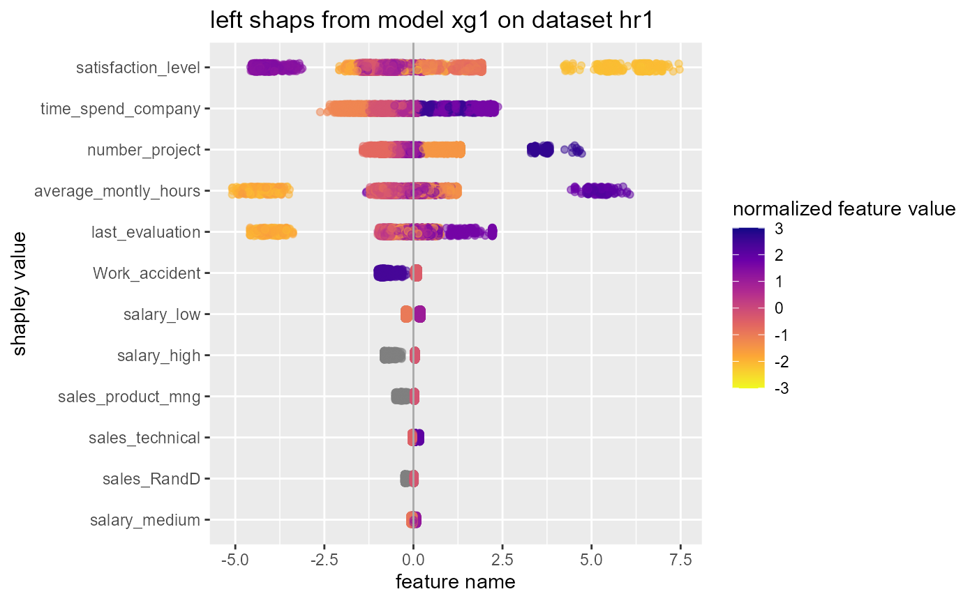
#>
#> $scatterplots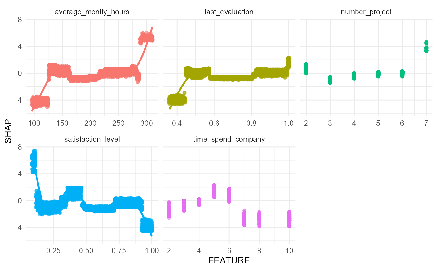
#>
#> $boxplots