TidyConsultant

knitr::opts_chunk$set(warning = FALSE, message = FALSE)
library(TidyConsultant)

In this vignette we demonstrate how the various packages in the TidyConsultant universe work together in a data science workflow by analyzing insurance data set, which consists of a population of people described by their characteristics and their insurance charge.

data(insurance)

Analyze data properties with validata

insurance %>% 
  diagnose()
#> # A tibble: 7 × 6
#>   variables types     missing_count missing_percent unique_count unique_rate
#>   <chr>     <chr>             <int>           <dbl>        <int>       <dbl>
#> 1 age       integer               0               0           47     0.0351 
#> 2 sex       character             0               0            2     0.00149
#> 3 bmi       numeric               0               0          548     0.410  
#> 4 children  integer               0               0            6     0.00448
#> 5 smoker    character             0               0            2     0.00149
#> 6 region    character             0               0            4     0.00299
#> 7 charges   numeric               0               0         1337     0.999

insurance %>% 
  diagnose_numeric()
#> # A tibble: 4 × 11
#>   variab…¹ zeros minus  infs    min   mean    max |x|<1…² integ…³   mode mode_…⁴
#>   <chr>    <int> <int> <int>  <dbl>  <dbl>  <dbl>   <dbl>   <dbl>  <dbl>   <dbl>
#> 1 age          0     0     0   18   3.92e1 6.4 e1   0     1   e+0   18   0.0516 
#> 2 bmi          0     0     0   16.0 3.07e1 5.31e1   0     2.24e-2   32.3 0.00972
#> 3 children   574     0     0    0   1.09e0 5   e0   0.429 1   e+0    0   0.429  
#> 4 charges      0     0     0 1122.  1.33e4 6.38e4   0     7.47e-4 1640.  0.00149
#> # … with abbreviated variable names ¹​variables, ²​`|x|<1 (ratio)`,
#> #   ³​integer_ratio, ⁴​mode_ratio

insurance %>% 
  diagnose_category(everything(),  max_distinct = 7) %>% 
  print(width = Inf)
#> # A tibble: 14 × 4
#>    column   level         n  ratio
#>    <chr>    <chr>     <int>  <dbl>
#>  1 sex      male        676 0.505 
#>  2 sex      female      662 0.495 
#>  3 children 0           574 0.429 
#>  4 children 1           324 0.242 
#>  5 children 2           240 0.179 
#>  6 children 3           157 0.117 
#>  7 children 4            25 0.0187
#>  8 children 5            18 0.0135
#>  9 smoker   no         1064 0.795 
#> 10 smoker   yes         274 0.205 
#> 11 region   southeast   364 0.272 
#> 12 region   northwest   325 0.243 
#> 13 region   southwest   325 0.243 
#> 14 region   northeast   324 0.242

We can infer that each row represents a person, uniquely identified by 5 characteristics. The charges column is also unique, but simply because it is a high-precision double.

insurance %>% 
  determine_distinct(everything())
#> database has 1 duplicate rows, and will eliminate them

Analyze data relationships with autostats

insurance %>% 
  auto_cor(sparse = TRUE) -> cors

cors
#> # A tibble: 20 × 6
#>    x                y              cor   p.value significance method 
#>    <chr>            <chr>        <dbl>     <dbl> <chr>        <chr>  
#>  1 smoker_no        charges    -0.787  8.27e-283 ***          pearson
#>  2 smoker_yes       charges     0.787  8.27e-283 ***          pearson
#>  3 charges          age         0.299  4.89e- 29 ***          pearson
#>  4 region_southeast bmi         0.270  8.71e- 24 ***          pearson
#>  5 charges          bmi         0.198  2.46e- 13 ***          pearson
#>  6 region_northeast bmi        -0.138  3.91e-  7 ***          pearson
#>  7 region_northwest bmi        -0.136  5.94e-  7 ***          pearson
#>  8 bmi              age         0.109  6.19e-  5 ***          pearson
#>  9 smoker_no        sex_female  0.0762 5.30e-  3 **           pearson
#> 10 smoker_no        sex_male   -0.0762 5.30e-  3 **           pearson
#> 11 smoker_yes       sex_female -0.0762 5.30e-  3 **           pearson
#> 12 smoker_yes       sex_male    0.0762 5.30e-  3 **           pearson
#> 13 region_southeast charges     0.0740 6.78e-  3 **           pearson
#> 14 region_southeast smoker_no  -0.0685 1.22e-  2 *            pearson
#> 15 region_southeast smoker_yes  0.0685 1.22e-  2 *            pearson
#> 16 charges          children    0.0680 1.29e-  2 *            pearson
#> 17 sex_female       charges    -0.0573 3.61e-  2 *            pearson
#> 18 sex_male         charges     0.0573 3.61e-  2 *            pearson
#> 19 sex_female       bmi        -0.0464 9.00e-  2 .            pearson
#> 20 sex_male         bmi         0.0464 9.00e-  2 .            pearson

Analyze the relationship between categorical and continuous variables

insurance %>% 
  auto_anova(everything(), baseline = "first_level") -> anovas1

anovas1 %>% 
  print(n = 50)
#> # A tibble: 32 × 12
#>    target   predictor level     estimate targe…¹     n std.e…² level_p…³ level…⁴
#>    <chr>    <chr>     <chr>        <dbl>   <dbl> <int>   <dbl>     <dbl> <chr>  
#>  1 age      region    (Interce…  3.93e+1  3.93e1   324 7.81e-1 4.75e-310 "***"  
#>  2 age      region    northwest -7.16e-2  3.92e1   325 1.10e+0 9.48e-  1 " "    
#>  3 age      region    southeast -3.29e-1  3.89e1   364 1.07e+0 7.59e-  1 " "    
#>  4 age      region    southwest  1.87e-1  3.95e1   325 1.10e+0 8.66e-  1 " "    
#>  5 age      sex       (Interce…  3.95e+1  3.95e1   662 5.46e-1 0         "***"  
#>  6 age      sex       male      -5.86e-1  3.89e1   676 7.68e-1 4.46e-  1 " "    
#>  7 age      smoker    (Interce…  3.94e+1  3.94e1  1064 4.31e-1 0         "***"  
#>  8 age      smoker    yes       -8.71e-1  3.85e1   274 9.52e-1 3.60e-  1 " "    
#>  9 bmi      region    (Interce…  2.92e+1  2.92e1   324 3.25e-1 0         "***"  
#> 10 bmi      region    northwest  2.63e-2  2.92e1   325 4.59e-1 9.54e-  1 " "    
#> 11 bmi      region    southeast  4.18e+0  3.34e1   364 4.47e-1 3.28e- 20 "***"  
#> 12 bmi      region    southwest  1.42e+0  3.06e1   325 4.59e-1 1.99e-  3 "**"   
#> 13 bmi      sex       (Interce…  3.04e+1  3.04e1   662 2.37e-1 0         "***"  
#> 14 bmi      sex       male       5.65e-1  3.09e1   676 3.33e-1 9.00e-  2 "."    
#> 15 bmi      smoker    (Interce…  3.07e+1  3.07e1  1064 1.87e-1 0         "***"  
#> 16 bmi      smoker    yes        5.67e-2  3.07e1   274 4.13e-1 8.91e-  1 " "    
#> 17 charges  region    (Interce…  1.34e+4  1.34e4   324 6.71e+2 7.67e- 78 "***"  
#> 18 charges  region    northwest -9.89e+2  1.24e4   325 9.49e+2 2.97e-  1 " "    
#> 19 charges  region    southeast  1.33e+3  1.47e4   364 9.23e+2 1.50e-  1 " "    
#> 20 charges  region    southwest -1.06e+3  1.23e4   325 9.49e+2 2.64e-  1 " "    
#> 21 charges  sex       (Interce…  1.26e+4  1.26e4   662 4.70e+2 1.63e-126 "***"  
#> 22 charges  sex       male       1.39e+3  1.40e4   676 6.61e+2 3.61e-  2 "*"    
#> 23 charges  smoker    (Interce…  8.43e+3  8.43e3  1064 2.29e+2 1.58e-205 "***"  
#> 24 charges  smoker    yes        2.36e+4  3.21e4   274 5.06e+2 8.27e-283 "***"  
#> 25 children region    (Interce…  1.05e+0  1.05e0   324 6.70e-2 1.26e- 50 "***"  
#> 26 children region    northwest  1.01e-1  1.15e0   325 9.47e-2 2.84e-  1 " "    
#> 27 children region    southeast  3.15e-3  1.05e0   364 9.21e-2 9.73e-  1 " "    
#> 28 children region    southwest  9.52e-2  1.14e0   325 9.47e-2 3.15e-  1 " "    
#> 29 children sex       (Interce…  1.07e+0  1.07e0   662 4.69e-2 2.66e- 98 "***"  
#> 30 children sex       male       4.14e-2  1.12e0   676 6.59e-2 5.30e-  1 " "    
#> 31 children smoker    (Interce…  1.09e+0  1.09e0  1064 3.70e-2 1.25e-147 "***"  
#> 32 children smoker    yes        2.29e-2  1.11e0   274 8.17e-2 7.79e-  1 " "    
#> # … with 3 more variables: predictor_p.value <dbl>,
#> #   predictor_significance <chr>, conclusion <chr>, and abbreviated variable
#> #   names ¹​target_mean, ²​std.error, ³​level_p.value, ⁴​level_significance
#> # ℹ Use `colnames()` to see all variable names

Use the sparse option to show only the most significant effects

insurance %>% 
  auto_anova(everything(), baseline = "first_level", sparse = T, pval_thresh = .1) -> anovas2

anovas2 %>% 
  print(n = 50)
#> # A tibble: 5 × 8
#>   target  predictor level      estimate target_mean     n level_p.value level_…¹
#>   <chr>   <chr>     <chr>         <dbl>       <dbl> <int>         <dbl> <chr>   
#> 1 bmi     region    southeast     4.18         33.4   364     3.28e- 20 ***     
#> 2 bmi     region    southwest     1.42         30.6   325     1.99e-  3 **      
#> 3 bmi     sex       male          0.565        30.9   676     9.00e-  2 .       
#> 4 charges sex       male       1387.        13957.    676     3.61e-  2 *       
#> 5 charges smoker    yes       23616.        32050.    274     8.27e-283 ***     
#> # … with abbreviated variable name ¹​level_significance

From this we can conclude that smokers and males incur higher insurance charges. It may be beneficial to explore some interaction effects, considering that BMI’s effect on charges will be sex-dependent.

create dummies out of categorical variables

insurance %>% 
  create_dummies(remove_most_frequent_dummy = T) -> insurance1

explore model-based variable contributions

insurance1 %>% 
  tidy_formula(target = charges) -> charges_form

charges_form
#> charges ~ age + bmi + children + sex_female + smoker_yes + region_northeast + 
#>     region_northwest + region_southwest
#> <environment: 0x0000016a9c2aeaa0>

insurance1 %>% 
  auto_variable_contributions(formula = charges_form)

insurance1 %>% 
  auto_model_accuracy(formula = charges_form)

create bins with tidybins

insurance1 %>% 
  bin_cols(charges) -> insurance_bins

insurance_bins
#> # A tibble: 1,338 × 10
#>    charges…¹   age   bmi child…² charges sex_f…³ smoke…⁴ regio…⁵ regio…⁶ regio…⁷
#>        <int> <int> <dbl>   <int>   <dbl>   <int>   <int>   <int>   <int>   <int>
#>  1         8    19  27.9       0  16885.       1       1       0       0       1
#>  2         1    18  33.8       1   1726.       0       0       0       0       0
#>  3         3    28  33         3   4449.       0       0       0       0       0
#>  4         9    33  22.7       0  21984.       0       0       0       1       0
#>  5         2    32  28.9       0   3867.       0       0       0       1       0
#>  6         2    31  25.7       0   3757.       1       0       0       0       0
#>  7         5    46  33.4       1   8241.       1       0       0       0       0
#>  8         4    37  27.7       3   7282.       1       0       0       1       0
#>  9         4    37  29.8       2   6406.       0       0       1       0       0
#> 10         9    60  25.8       0  28923.       1       0       0       1       0
#> # … with 1,328 more rows, and abbreviated variable names ¹​charges_fr10,
#> #   ²​children, ³​sex_female, ⁴​smoker_yes, ⁵​region_northeast, ⁶​region_northwest,
#> #   ⁷​region_southwest
#> # ℹ Use `print(n = ...)` to see more rows

Here we can see a summary of the binned cols. The with quintile “value” bins we can see that the top 20% of charges comes from the top x people.

insurance_bins %>% 
  bin_summary()
#> # A tibble: 10 × 14
#>    column method n_bins .rank   .min  .mean   .max .count .uniq…¹ relat…²   .sum
#>    <chr>  <chr>   <int> <int>  <dbl>  <dbl>  <dbl>  <int>   <int>   <dbl>  <dbl>
#>  1 charg… equal…     10    10 34806. 42267. 63770.    136     136  100    5.75e6
#>  2 charg… equal…     10     9 20421. 26063. 34780.    130     130   61.7  3.39e6
#>  3 charg… equal…     10     8 13823. 16757. 20297.    135     135   39.6  2.26e6
#>  4 charg… equal…     10     7 11412. 12464. 13770.    134     134   29.5  1.67e6
#>  5 charg… equal…     10     6  9386. 10416. 11397.    134     134   24.6  1.40e6
#>  6 charg… equal…     10     5  7372.  8386.  9378.    134     134   19.8  1.12e6
#>  7 charg… equal…     10     4  5484.  6521.  7358.    134     134   15.4  8.74e5
#>  8 charg… equal…     10     3  3994.  4752.  5478.    133     133   11.2  6.32e5
#>  9 charg… equal…     10     2  2353.  3140.  3990.    134     134    7.43 4.21e5
#> 10 charg… equal…     10     1  1122.  1797.  2332.    134     133    4.25 2.41e5
#> # … with 3 more variables: .med <dbl>, .sd <dbl>, width <dbl>, and abbreviated
#> #   variable names ¹​.uniques, ²​relative_value
#> # ℹ Use `colnames()` to see all variable names

Create and analyze xgboost model for binary classification

Let’s see if we can predict whether a customer is a smoker.

Xgboost considers the first level of a factor to be the “positive event” so let’s ensure that “yes” is the first level using framecleaner::set_fct

insurance %>% 
  set_fct(smoker, first_level = "yes") -> insurance

insurance %>% 
  create_dummies(where(is.character), remove_first_dummy = T) -> insurance_dummies

insurance_dummies %>% 
  diagnose
#> # A tibble: 9 × 6
#>   variables        types   missing_count missing_percent unique_count unique_r…¹
#>   <chr>            <chr>           <int>           <dbl>        <int>      <dbl>
#> 1 age              integer             0               0           47    0.0351 
#> 2 bmi              numeric             0               0          548    0.410  
#> 3 children         integer             0               0            6    0.00448
#> 4 smoker           factor              0               0            2    0.00149
#> 5 charges          numeric             0               0         1337    0.999  
#> 6 sex_male         integer             0               0            2    0.00149
#> 7 region_northwest integer             0               0            2    0.00149
#> 8 region_southeast integer             0               0            2    0.00149
#> 9 region_southwest integer             0               0            2    0.00149
#> # … with abbreviated variable name ¹​unique_rate

And create a new formula for the binary classification.

insurance_dummies %>% 
  tidy_formula(target = smoker) -> smoker_form

smoker_form
#> smoker ~ age + bmi + children + charges + sex_male + region_northwest + 
#>     region_southeast + region_southwest
#> <environment: 0x0000016aa56b3ed0>

Now we can create a basic model using tidy_xgboost. Built in heuristic will automatically recognize this as a binary classification task. We can tweak some parameters to add some regularization and increase the number of trees. Xgboost will automatically output feature importance on the training set, and a measure of accuracy tested on a validation set.

insurance_dummies %>% 
  tidy_xgboost(formula = smoker_form, 
              mtry = .5,
              trees = 100L,
              loss_reduction = 1,
              alpha = .1,
              sample_size = .7) -> smoker_xgb_classif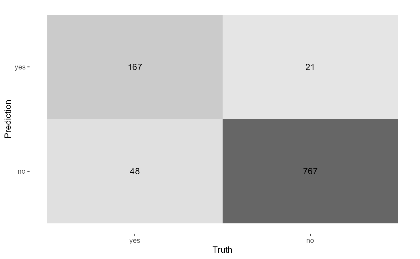

#> # A tibble: 15 × 3
#>    .metric              .estimate .formula              
#>    <chr>                    <dbl> <chr>                 
#>  1 accuracy                 0.931 TP + TN / total       
#>  2 kap                      0.786 NA                    
#>  3 sens                     0.777 TP / actually P       
#>  4 spec                     0.973 TN / actually N       
#>  5 ppv                      0.888 TP / predicted P      
#>  6 npv                      0.941 TN / predicted N      
#>  7 mcc                      0.789 NA                    
#>  8 j_index                  0.750 NA                    
#>  9 bal_accuracy             0.875 sens + spec / 2       
#> 10 detection_prevalence     0.187 predicted P / total   
#> 11 precision                0.888 PPV, 1-FDR            
#> 12 recall                   0.777 sens, TPR             
#> 13 f_meas                   0.829 HM(ppv, sens)         
#> 14 baseline_accuracy        0.786 majority class / total
#> 15 roc_auc                  0.987 NA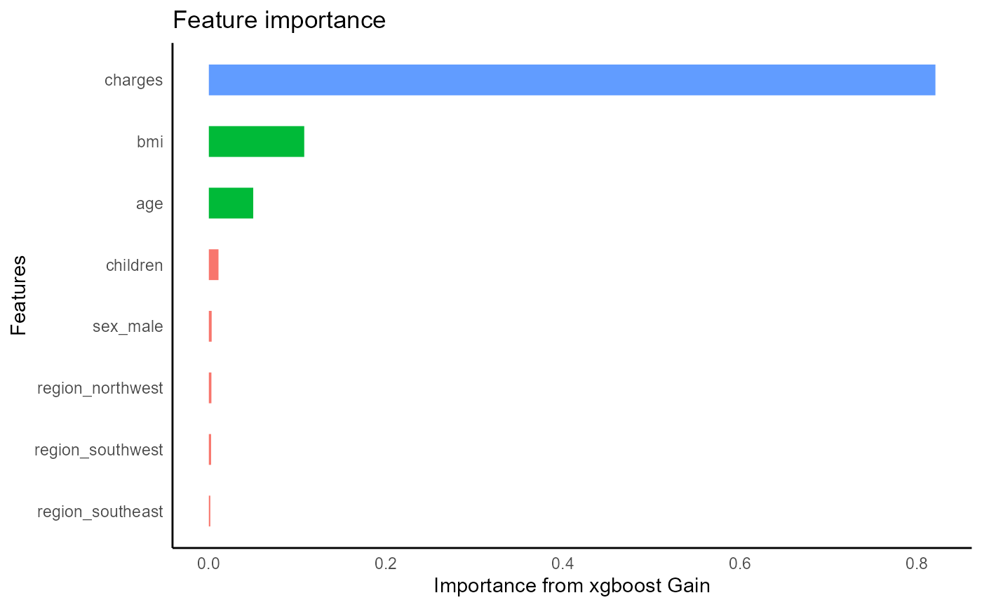

Obtain predictions

smoker_xgb_classif %>% 
  tidy_predict(newdata = insurance_dummies, form = smoker_form) -> insurance_fit

Analyze the probabilities using tidybins. We can find the top 20% of customers most likely to be smokers.

names(insurance_fit)[length(names(insurance_fit)) - 1] -> prob_preds

insurance_fit %>% 
  bin_cols(prob_preds, n_bins = 5) -> insurance_fit1

insurance_fit1 %>% 
  bin_summary()
#> # A tibble: 5 × 14
#>   column      method n_bins .rank    .min   .mean    .max .count .uniq…¹ relat…²
#>   <chr>       <chr>   <int> <int>   <dbl>   <dbl>   <dbl>  <int>   <int>   <dbl>
#> 1 smoker_pre… equal…      5     5 7.12e-1 9.63e-1 9.98e-1    268     253 96.3   
#> 2 smoker_pre… equal…      5     4 1.51e-3 5.57e-2 6.84e-1    267     243  5.57  
#> 3 smoker_pre… equal…      5     3 5.77e-4 9.50e-4 1.50e-3    272     221  0.0950
#> 4 smoker_pre… equal…      5     2 3.14e-4 4.34e-4 5.76e-4    261     199  0.0434
#> 5 smoker_pre… equal…      5     1 1.27e-4 2.34e-4 3.13e-4    270     190  0.0234
#> # … with 4 more variables: .sum <dbl>, .med <dbl>, .sd <dbl>, width <dbl>, and
#> #   abbreviated variable names ¹​.uniques, ²​relative_value
#> # ℹ Use `colnames()` to see all variable names

Evaluate the training error. eval_preds uses both the probability estimates and binary estimates to calculate a variety of metrics.

insurance_fit1 %>% 
  eval_preds()
#> # A tibble: 4 × 5
#>   .metric   .estimator .estimate model              target
#>   <chr>     <chr>          <dbl> <chr>              <chr> 
#> 1 accuracy  binary         0.998 smoker_xgb_classif smoker
#> 2 f_meas    binary         0.995 smoker_xgb_classif smoker
#> 3 precision binary         0.993 smoker_xgb_classif smoker
#> 4 roc_auc   binary         1.00  smoker_xgb_classif smoker

Traditional yardstick confusion matrix can be created manually.

names(insurance_fit)[length(names(insurance_fit))] -> class_preds

insurance_fit1 %>% 
  yardstick::conf_mat(truth = smoker, estimate = class_preds) -> conf_mat_sm

conf_mat_sm
#>           Truth
#> Prediction  yes   no
#>        yes  273    2
#>        no     1 1062