autostats

library(autostats)

plot variable contributions

multiclass target

Species is a 3-level factor so it will be automatically modelled with a multiclass neural network and a light gbm with multiclass objective function.

First set define the formula to use for modeling.

iris %>% 
  tidy_formula(target = Species) -> species_formula

species_formula
#> Species ~ Sepal.Length + Sepal.Width + Petal.Length + Petal.Width
#> <environment: 0x0000018c1f320008>

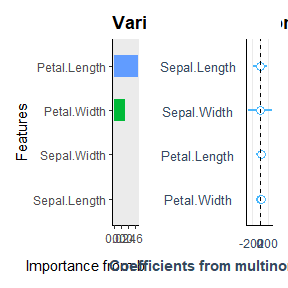
iris %>% 
  auto_variable_contributions(species_formula)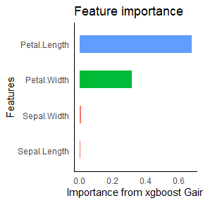

iris %>% 
  auto_model_accuracy(species_formula)

binary target

Linear models uses weighted logistic regression for modeling the coefficients

iris %>% 
  filter(Species != "setosa") %>% 
  auto_variable_contributions(species_formula)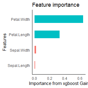

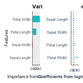
For the variable contributions the linear model uses penalized logistic regression provided by glmnet.

iris %>% 
  filter(Species != "setosa") -> iris_binary

iris_binary %>% 
  auto_model_accuracy(species_formula)

continuous target

Models are automatically adapted for a continuous target.

Define the new formula

iris %>% 
  tidy_formula(target = Petal.Length) -> petal_formula

petal_formula
#> Petal.Length ~ Sepal.Length + Sepal.Width + Petal.Width + Species
#> <environment: 0x0000018c276dae50>

iris %>% 
  auto_model_accuracy(petal_formula)

auto anova

auto anova automatically regresses each continuous variable supplied against each categorical variable supplied. Lm is called separately for each continuous/ categorical variable pair, but the results are reported in one dataframe. Whether the outcome differs amongst categorical levels is determined by the p.value. The interpretation is affected by the choice of baseline for comparison. Traditionally the first level of the factor is used, however option to use the mean of the continuous variable as the baseline intercept is a helpful comparison.

iris %>% 
  auto_anova(Species, matches("Petal"), baseline = "first_level")
#> # A tibble: 6 × 12
#>   target   predi…¹ level estim…² targe…³     n std.e…⁴ level_…⁵ level…⁶ predic…⁷
#>   <chr>    <chr>   <chr>   <dbl>   <dbl> <int>   <dbl>    <dbl> <chr>      <dbl>
#> 1 Petal.L… Species (Int…   1.46    1.46     50  0.0609 9.30e-53 ***     2.86e-91
#> 2 Petal.L… Species vers…   2.80    4.26     50  0.0861 5.25e-69 ***     2.86e-91
#> 3 Petal.L… Species virg…   4.09    5.55     50  0.0861 4.11e-91 ***     2.86e-91
#> 4 Petal.W… Species (Int…   0.246   0.246    50  0.0289 1.96e-14 ***     4.17e-85
#> 5 Petal.W… Species vers…   1.08    1.33     50  0.0409 1.25e-57 ***     4.17e-85
#> 6 Petal.W… Species virg…   1.78    2.03     50  0.0409 7.95e-86 ***     4.17e-85
#> # … with 2 more variables: predictor_significance <chr>, conclusion <chr>, and
#> #   abbreviated variable names ¹​predictor, ²​estimate, ³​target_mean, ⁴​std.error,
#> #   ⁵​level_p.value, ⁶​level_significance, ⁷​predictor_p.value
#> # ℹ Use `colnames()` to see all variable names