library(autostats)
library(workflows)
library(dplyr)
library(tune)
library(rsample)
library(hardhat)
autostats provides convenient wrappers for modeling,
visualizing, and predicting using a tidy workflow. The emphasis is on
rapid iteration and quick results using an intuitive interface based off
the tibble and tidy_formula.
Prepare data
Set up the iris data set for modeling. Create dummies and any new columns before making the formula. This way the same formula can be use throughout the modeling and prediction process.
set.seed(34)

 iris %>%
  dplyr::as_tibble() %>%
  framecleaner::create_dummies(remove_first_dummy  = TRUE) -> iris1
#> 1 column(s) have become 2 dummy columns

 iris1 %>%
 tidy_formula(target = Petal.Length) -> petal_form

 petal_form
#> Petal.Length ~ Sepal.Length + Sepal.Width + Petal.Width + Species_versicolor +
#>     Species_virginica
#> <environment: 0x0000023ae35330b0>
Use the rsample package to split into train and validation sets.
iris1 %>%
  rsample::initial_split() -> iris_split

iris_split %>%
  rsample::analysis() -> iris_train

iris_split %>%
  rsample::assessment() -> iris_val

iris_split
#> <Training/Testing/Total>
#> <112/38/150>
Fit boosting models and visualize
Fit models to the training set using the formula to predict
Petal.Length. Variable importance using gain for each
xgboost model can be visualized.
xgboost with bayesian hyperparameter optimization
auto_tune_xgboost returns a workflow object with tuned
parameters and requires some postprocessing to get a traind
xgb.Booster object like tidy_xgboost. Tuning
iterations set to 1 just so the vignette builds quickly.
Default is n_iter = 100
iris_train %>%
  auto_tune_xgboost(formula = petal_form, n_iter = 7L, tune_method = "bayes") -> xgb_tuned_bayes

xgb_tuned_bayes %>%
  parsnip::fit(iris_train) %>%
  hardhat::extract_fit_engine() -> xgb_tuned_fit_bayes

xgb_tuned_fit_bayes %>%
  visualize_model()
xgboost with grid search hyperparameter optimization
xgboost also can be tuned using a grid that is created
internally using dials::grid_max_entropy. The
n_iter parameter is passed to grid_size.
Parallelization is highly effective in this method, so the default
argument parallel = TRUE is recommended.
iris_train %>%
  auto_tune_xgboost(formula = petal_form, n_iter = 5L,trees = 20L, loss_reduction = 2, mtry = .5, tune_method = "grid", parallel = FALSE) -> xgb_tuned_grid

xgb_tuned_grid %>%
  parsnip::fit(iris_train) %>%
  parsnip::extract_fit_engine() -> xgb_tuned_fit_grid

xgb_tuned_fit_grid %>%
  visualize_model()
xgboost with default parameters
iris_train %>%
  tidy_xgboost(formula = petal_form) -> xgb_base
#> accuracy tested on a validation set
#> # A tibble: 3 × 2
#>   .metric .estimate
#>   <chr>       <dbl>
#> 1 ccc         0.975
#> 2 rmse        0.375
#> 3 rsq         0.953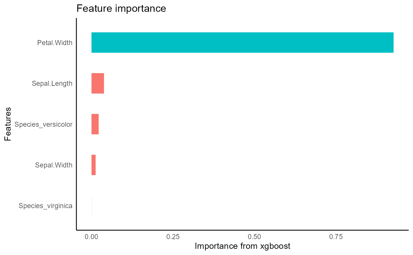
xgb_base %>%
  visualize_model()
xgboost with hand-picked parameters
iris_train %>%
  tidy_xgboost(petal_form,
               trees = 250L,
               tree_depth = 3L,
               sample_size = .5,
               mtry = .5,
               min_n = 2) -> xgb_opt
#> accuracy tested on a validation set
#> # A tibble: 3 × 2
#>   .metric .estimate
#>   <chr>       <dbl>
#> 1 ccc         0.979
#> 2 rmse        0.347
#> 3 rsq         0.964
xgb_opt %>%
  visualize_model()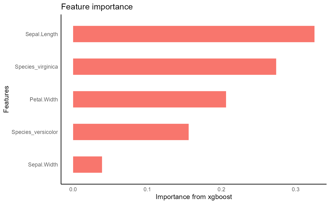
agtboost
automated gradient descent boosting with information-criterion heuristics that don’t need tuning
iris_train %>%
  tidy_agtboost(petal_form) -> agtb
#> no dummies were created
predict on validation set
make predictions
Predictions are iteratively added to the validation data frame. The name of the column is automatically created using the models name and the prediction target.
xgb_base %>%
  tidy_predict(newdata = iris_val, form = petal_form) -> iris_val2
#> created the following column: Petal.Length_preds_xgb_base

xgb_opt %>%
  tidy_predict(newdata = iris_val2, petal_form) -> iris_val3
#> created the following column: Petal.Length_preds_xgb_opt

agtb %>%
    tidy_predict(newdata = iris_val3, petal_form)-> iris_val4

iris_val4 %>%
  names()
#> [1] "Sepal.Length"                "Sepal.Width"
#> [3] "Petal.Length"                "Petal.Width"
#> [5] "Species_versicolor"          "Species_virginica"
#> [7] "Petal.Length_preds_xgb_base" "Petal.Length_preds_xgb_opt"
#> [9] "Petal.Length_preds_agtb"
predictions with eval_preds
Instead of evaluationg these prediction 1 by 1, This step is
automated with eval_preds. This function is specifically
designed to evaluate predicted columns with names given from
tidy_predict.
iris_val4 %>%
  eval_preds()
#> # A tibble: 9 × 5
#>   .metric .estimator .estimate model    target
#>   <chr>   <chr>          <dbl> <chr>    <chr>
#> 1 ccc     standard       0.983 agtb     Petal.Length
#> 2 ccc     standard       0.980 xgb_base Petal.Length
#> 3 ccc     standard       0.984 xgb_opt  Petal.Length
#> 4 rmse    standard       0.319 agtb     Petal.Length
#> 5 rmse    standard       0.352 xgb_base Petal.Length
#> 6 rmse    standard       0.312 xgb_opt  Petal.Length
#> 7 rsq     standard       0.975 agtb     Petal.Length
#> 8 rsq     standard       0.969 xgb_base Petal.Length
#> 9 rsq     standard       0.972 xgb_opt  Petal.Length
get shapley values
tidy_shap has similar syntax to
tidy_predict and can be used to get shapley values from
xgboost models on a validation set.
shap_list$shap_tbl
#> # A tibble: 38 × 5
#>    Sepal.Length Sepal.Width Petal.Width Species_versicolor Species_virginica
#>           <dbl>       <dbl>       <dbl>              <dbl>             <dbl>
#>  1       -0.236     -0.0700       -1.97             0.0970          0.000452
#>  2       -0.284     -0.0764       -2.02             0.0954          0.000395
#>  3       -0.118     -0.0969       -2.04             0.0970          0.00137
#>  4       -0.244     -0.0778       -1.99             0.0970          0.000452
#>  5       -0.143     -0.0595       -2.08             0.0970          0.000452
#>  6       -0.281     -0.0627       -2.01             0.0970          0.000845
#>  7       -0.228     -0.0395       -1.90             0.0970          0.000856
#>  8       -0.260     -0.145        -2.04             0.0954          0.000351
#>  9       -0.223     -0.0909       -1.99             0.0954          0.000395
#> 10       -0.281      0.272        -1.86             0.0960         -0.00104
#> # … with 28 more rows
#> # ℹ Use `print(n = ...)` to see more rows
shap_list$shap_summary
#> # A tibble: 5 × 5
#>   name                  cor       var     sum sum_abs
#>   <chr>               <dbl>     <dbl>   <dbl>   <dbl>
#> 1 Petal.Width         0.955 2.29       8.43    53.7
#> 2 Sepal.Length        0.809 0.0875    -2.27     7.82
#> 3 Species_versicolor -0.934 0.0333     3.33     7.20
#> 4 Sepal.Width        -0.696 0.0148     0.310    3.25
#> 5 Species_virginica  -0.326 0.0000230 -0.0427   0.107
shap_list$swarmplot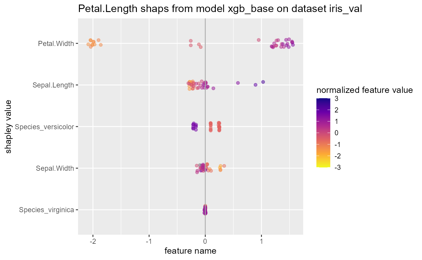
shap_list$scatterplotsunderstand xgboost with other functions from the original package
Overfittingin the base config may be related to growing deep trees.
 xgb_base %>%
  xgboost::xgb.plot.deepness()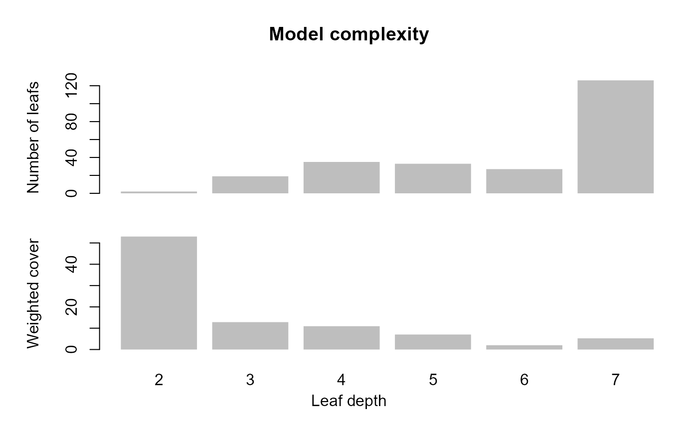
 xgb_base %>%
  xgboost::xgb.plot.deepness()
Plot the first tree in the model. The small in terminal leaves suggests
overfitting in the base model.
Plot the first tree in the model. The small in terminal leaves suggests
overfitting in the base model.
xgb_base %>%
  xgboost::xgb.plot.tree(model = ., trees = 1)